2018年5月14日 星期一

Notes on applying the LSTM in Computer Vision

Overview

  This article illustrates several key points while applying the CNN with the LSTM in Computer Vision.

Introduction

  Nowadays, the Convolutional Neural Network (CNN) shows its great successes in many computer vision tasks, such as the image classification, the object detection, and the object segmentation... etc.  However, most of these algorithms are only be able to apply on the image (or, the single frame).  For example, most of the object detectors can detect and highlight the car which drives along the road.  Since the object detector is designed to detect the car in a single frame (i.e. it cannot take temporal information into consideration), the object detector may fail to detect the car while it is currently occluded by a tree.  However, we can still expect the position of the car because the human brain takes the history of the interested object into consideration.
  To overcome such issue, it's very intuitive to combine the CNN and the LSTM.  However, there are several tricks to be noted when applying the LSTM in computer vision.

Notes:

1. Adding dropout and regularization

  The LSTM is as easy as the fully-connected layer to get overfitting, not to mention that the LSTM can be seen as the 4 layers combination of the fully-connected layer.
  Fortunately, the TensorFlow provides the dropout wrapper for LSTM that can perform the dropout between the stacked LSTM (Note: this paper states that it'd be better to use dropout between the LSTM cells than use inside the cell.).  See this website for more detail.
  For the regularization, you need to get all of the variables first, then filter the variables of LSTM out by the name scope.  See this website for more detail.
  Finally, the wrapper function of LSTM is defined as follows:
def LSTM(name_, inputTensor_, numberOfOutputs_, isTraining_, dropoutProb_=None):
 with tf.name_scope(name_):
  cell = tf.nn.rnn_cell.LSTMCell(num_units=numberOfOutputs_,
       use_peepholes=True,
       initializer=layerSettings.LSTM_INITIALIZER,
       forget_bias=1.0,
       state_is_tuple=True,
       activation=tf.nn.tanh,
       name=name_+"_cell")

  if dropoutProb_ != None:
   dropoutProbTensor = tf.cond(isTraining_, lambda: dropoutProb_, lambda: 1.0)
   cell = tf.nn.rnn_cell.DropoutWrapper(cell,
            input_keep_prob=dropoutProbTensor,
            output_keep_prob=dropoutProbTensor)

  statePlaceHolder = tf.nn.rnn_cell.LSTMStateTuple( tf.placeholder(layerSettings.FLOAT_TYPE, [None, numberOfOutputs_]),
          tf.placeholder(layerSettings.FLOAT_TYPE, [None, numberOfOutputs_]) )

  outputTensor, stateTensor = tf.nn.dynamic_rnn( cell=cell,
        initial_state=statePlaceHolder,
        inputs=inputTensor_)

  # Add Regularization Loss
  for eachVariable in tf.trainable_variables():
   if name_ in eachVariable.name:
    if ('bias' not in eachVariable.name)and(layerSettings.REGULARIZER_WEIGHTS_DECAY != None):
     regularizationLoss = L2_Regularizer(eachVariable)
     tf.losses.add_loss(regularizationLoss, loss_collection=tf.GraphKeys.REGULARIZATION_LOSSES)
     

 return outputTensor, stateTensor, statePlaceHolder

2. Unrolls the LSTM

  In training the single frame algorithms, the batch data will be the shape: (batch_size, w, h, c).  While training the video algorithms, the batch data will be the shape: (batch_size, unrolled_size, w, h, c).  Here, the batch_size means how many videos in this batch while the unrolled_size means how many frames per video.
  By applying the tf.nn.dynamic_rnn(), which takes the input tensor and the LSTM cell as arguments, it will unroll the input in the second dimension and feed it into the LSTM cell.

3. Start training with a few Unroll Size

  Several studies (such as Re3 and here) show that one should start with a larger batch_size and a smaller unroll_size while training the network with the LSTM.  Otherwise, the network will not converge.  Namely, the user should start with a bunch of videos (say 40 videos, for example), but with a few frames (say 2 frames per video, for example).  Then double the number of unrolls and halve the batch_size while the network reaches the loss plateaus, as suggested by the Re3.  For example, input 20 videos and 4 frames per video while the network reaches the first plateau.
  Nonetheless, the above situation does not occur in my recent project:  Without the use of above method, the network still converges easily.  And the use of the above method does not improve the network to converge to the lower minima as well.  However, I think it's still advantageous for one to start training with the above method.

4. Which should be fed into the current network: the output or the label of the previous time?

  In the deploying time of NLP, the output of the previous frame should also be inputted to the network, as shown in the following figure.

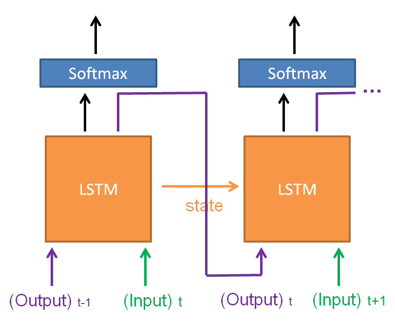
In training, however, the label of the previous frame should be inputted instead, as shown follows.
  Normally, the above mechanism has not been applied in computer vision.  However, in some special cases, this mechanism is also applied.  For example, in Re3, the user is asked to drag a bounding box of an interested object.
  The Re3 network will track the object in the next frame by input two cropped images:  The first cropped image is an image in the previous frame that cropped by the bounding box of the interested object (actually, it is as twice the size as the bounding box).  The second cropped image is a sub-image that cropped in the same way as the first cropped image (i.e. the same (x, y, w, h) as the previous crop), but apply on the current frame image.  The output of the network is the bounding box of the interested object in the current frame.  The current frame is then cropped by such output bounding box and will be used as the previous frame for the next run.
  The way to crop the current frame is similar to the mechanism shown in the above figure: During deploying, the crop coordinate of the current frame is determined by the previous output.  However, one should use the previous label of bounding box while training and slightly increase the probability to use the previous output after some condition met.  In Re3, the probability of using the previous label starts with 0 than plus 0.25 while the user increases the unroll size.

5. The cell state of the LSTM should be maintained in a different way while train and deploy, respectively.
  While training the LSTM, the cell state is reset to zeros per video.  Suppose that the input batch is of the shape: (b, u, w, h, c) and the LSTM has N neurons, one should create the initial cell state as:
 initialCellState = tuple( [np.zeros([b, N])] * 2 )
 initialCellState = tf.nn.rnn_cell.LSTMStateTuple(initialCellState[0], initialCellState[1])
Note that the initialCellState includes both the hidden state and the output state.

  While deploying, the cell state should be maintained and then pass to the feed_dict each frame by the user.  Furthermore, the user should get the value of the LSTM states by sess.run() the state tensor of the LSTM.  The deploying procedure looks like:
  inputFeedDict = { self.net.inputImage : batchData.batchOfImages,
      ...
      self.net.isTraining : False
    }
  cellStateFeedDict = self.net.GetFeedDictOfLSTM(...)

  inputFeedDict.update(cellStateFeedDict)

  loss, listOfPreviousCellStates = session.run( [ self._lossOp] + self.net.GetListOfStatesTensorInLSTMs(),
                            feed_dict = inputFeedDict )

To decouple the train/deploy from the network design, I define the interface of the networks as follows:
class NetworkBase:
 __metaclass__ = ABCMeta
 @abstractmethod
 def Build(self):
  pass

 @abstractmethod
 def GetListOfStatesTensorInLSTMs(self):
  pass

 @abstractmethod
 def GetFeedDictOfLSTM(self, BATCH_SIZE_, listOfPreviousStateValues_=None):
  pass
And one possible implementation of a network that contains one LSTM is shown as follows (see here for more detail):
class Net(NetworkBase):
 def __init__(...):
  ...

 def Build(self):
  ...

  out, self._stateTensorOfLSTM_1, self._statePlaceHolderOfLSTM_1 = LSTM( "LSTM_1",
           out,
           self._NUMBER_OF_NEURONS_IN_LSTM,
           isTraining_=self._isTraining,
           dropoutProb_=self._DROPOUT_PROB)
  ...


 def GetListOfStatesTensorInLSTMs(self):
  return [self._stateTensorOfLSTM_1]


 def GetFeedDictOfLSTM(self, BATCH_SIZE_, listOfPreviousStateValues_=None):
  if listOfPreviousStateValues_ == None:
   '''
       For the first time (or, the first of Unrolls), there's no previous state,
       return zeros state.
   '''
   initialCellState = tuple( [np.zeros([BATCH_SIZE_, self._NUMBER_OF_NEURONS_IN_LSTM])] * 2 )
   initialCellState = tf.nn.rnn_cell.LSTMStateTuple(initialCellState[0], initialCellState[1])

   return {self._statePlaceHolderOfLSTM_1 : initialCellState }

  else:
   return { self._statePlaceHolderOfLSTM_1 : listOfPreviousStateValues_[0] }

Therefore, in training, one could just (see here for more detail):
  inputFeedDict = { self.net.inputImage : batchData.batchOfImages,
      ...
      self.net.isTraining : True,
    }

  '''
      For Training, do not use previous state.  Set the argument:
      'listOfPreviousStateValues_'=None to ensure using the zeros
      as LSTM state.
  '''
  cellStateFeedDict = self.net.GetFeedDictOfLSTM(batchData.batchSize, listOfPreviousStateValues_=None)
  inputFeedDict.update(cellStateFeedDict)

  session_.run( [self._optimzeOp],
         feed_dict = inputFeedDict )
While in deploying, one could simply (see here for more detail):
  inputFeedDict = { self.net.inputImage : batchData.batchOfImages,
      ...
      self.net.isTraining : False,
    }
  cellStateFeedDict = self.net.GetFeedDictOfLSTM(batchData.batchSize, self._listOfPreviousCellState)

  inputFeedDict.update(cellStateFeedDict)

  tupleOfOutputs = session.run( [ self._lossOp] + self.net.GetListOfStatesTensorInLSTMs(),
                feed_dict = inputFeedDict )
  listOfOutputs = list(tupleOfOutputs)
  batchLoss = listOfOutputs.pop(0)
  self._listOfPreviousCellState = listOfOutputs

6. Gradient Clipping

  It's well known that the LSTM suffer from gradient explosion.  Therefore, the gradients are often examined and clipped to a certain range.  See here for gradient clipping in TensorFlow.
  In Re3, they state that it is not necessary to clip the gradients if one applies the training strategy that starts with a few unrolls.  However, in my recent project, the exploding gradients happened even if I apply such training strategy.

2018年5月4日 星期五

Violence Detection by CNN + LSTM

Overview

  This article shows the detail of my currently developed project: Violence Detection.  The proposed approach outperforms the state-of-the-art methods, while still processing the videos in real-time.  The comparison between my method and the previous work by Conv3D is also shown.


Introduction

  School fight is always a big issue while I was guarding the high school.  However, to monitor the surveillance cameras by staffs is infeasible, not to mention they may have other responsibilities.  Fortunately, the currently raised AI (or, the Deep Learning) techniques may be able to detect the anomalies automatically [1].  Such anomaly detection is very fast and can be used as the preprocessing to filter out the normal surveillance videos, and then send the anomaly videos to perform the further examinations by other highly accurate algorithms.
  The previous work on violence detection use traditional features such as the BoVW, the STIP, and the MoSIFT, and classify the features by SVM [2].  Ding et. al. extract the spatial and temporal features by the 3D convolution layers and classify the features by the fully-connected layers (as shown in Fig. 1) [3].  However, both of the proposed methods do not well support the variable length of videos.  And the computational time of 3D convolution grows rapidly because of the depth of the temporal axis.


Fig. 1.  Violence detection by 3D convolutional networks in ref. [3].


  Moreover, the lack of the richness of the large-scale video dataset is also an issue.  Although the Sports-1M dataset [4] provides a million of videos, most of the categories are about sports (i.e. The diversity of the videos is not as rich as the ImageNet).  However, several studies imply that if the pre-trained model had seen a certain object that will be used later in the transfer learning task, the performance of the target task will be better [4, 5].  Therefore, the availability of the use of the pre-trained model on ImageNet is also important, not to mention that there are plenty amounts of available pre-trained models.
  In this work, a new network is proposed:  A CNN takes the input video frames and outputs the features to the Long Short-Term Memory (LSTM) to learn global temporal features and finally classify the features by fully-connected layers.  This network can not only implement by the pre-trained models in ImageNet, but also have the flexibility to accept variable length videos, and even boosts the accuracy to the 98.5% while still processing the image in real-time (80 fps on Nvidia GTX 1080 Ti).


Method

Network Architecture

  The proposed network architecture is shown in Fig. 2.  It has been shown that in addition to adding the LSTM (which is supposed to extract global temporal features) after the CNN, the local temporal features that can be obtained from the optical flow is also important [6].  Furthermore, it has been reported that the virtue of the optical flow is due to its invariance in appearance as well as its accurate at boundaries and at small displacements [7].  Therefore, in this work, the effect of optical flow is supposed to be mimicked by taking two video frames as input.  The two input frames are processed by the pre-trained CNN.  The two frames outputs from the bottom layer of the pre-trained model are concatenated in the last channel and then fed into the additional CNN (labeled by orange color in Fig. 2).  Since the outputs from the bottom layer are regarded as the low-level features, the additional CNN is supposed to learn the local motion features as well as the appearance invariant features by comparing the two frames feature map.  The two frames outputs from the top layer of the pre-trained network are also concatenated and fed into the other additional CNN to compare the high-level features of the two frames.  The outputs from the two additional CNN are then concatenated and passed to a fully-connected layer and the LSTM cell to learn the global temporal features.  Finally, the outputs of the LSTM cell are classified by a fully-connected layer which contained two neurons that represent the two categories (fight and non-fight), respectively.


Fig. 2.  The proposed network architecture.  The layers that labeled by blue color are pre-trained on the ImageNet dataset and are frozen during training.  The layers that labeled by the orange color are trained on the video dataset.


  The pre-trained model is implemented by Darknet19 [8] due to its accuracy on ImageNet and the above real-time performance.  Since the Darknet19 already contains 19 convolutional layers, to avoid the degradation problem [9], the additional CNN are implemented by the residual layers [9].

Accuracy Evaluation

  The proposed model in this work can output the classified result per frame.  However, the previous research evaluates the accuracy at the video-level.  To be able to compare with the previous work, the frame-level results are gathered and processed by the following strategy:  The video is classified to a certain category if and only if the number of the continuous signals of such category is larger than a certain threshold.  Such threshold can be derived by scanning the threshold from 0 to the length of the video and see which threshold yields the best accuracy in the validation set, as shown in Fig. 3.  If there are multiple thresholds that can yield the same accuracy, the small one will be chosen.


Fig. 3.  The threshold-accuracy curve in the validation set.  The horizontal axis represents the threshold of the number of continuous frames that has the positive signal.  The vertical axis represents the accuracy at such threshold in the validation set.  In the figure, thresholds start from 3 to 9 are all yield the best accuracy.  The smallest threshold (i.e. threshold = 3) is chosen so that the continuous false positive in the test set could be reflected by this metric.

Gradient Clipping

  It is well known that the gradient of the recurrent network may increase rapidly due to the long-term components [10].  The normal way to deal with the exploding gradient would be: truncate the gradient so that it remains in a reasonable range.  While several studies solve this issue by another approach: start training with few unrolls, and then double the size of unrolls when the loss reaches plateaus [5].  In the second approach, they found that it even not necessary to clip the gradients.  They also state that without starting from the small unrolls, the network may not even converge [5].
  In this work, I found that the network can easily converge even the initial unrolls is set to the length of the videos.  However, the absence of the gradient clipping makes the loss curve oscillating during training even if the training is starting with a small unrolls.  Therefore, the gradients of the network are truncated in the range from -5.0 to 5.0.  Clipping the gradients into the smaller range (e.g. from -1.0 to 1.0) has also been tested.  However, my experiment shows that this will cause the network hardly to converge to the lower minima.


Results

Experiment on the Hockey dataset

  The Hockey dataset proposed by Bermejo et. al. has 500 fighting clips and 500 non-fighting clips collected from the hockey games [2].  Follow the experiment proposed by Ding et. al. [3], the dataset is further split into the following configuration: the 400 clips (including 200 fighting clips and 200 non-fighting clips)  for testing, the 500 clips for training and the 100 clips for validation.  The result is shown in Table 1.  One can see that the proposed method in this work outperforms other state-of-the-art methods.


Method
Accuracy
STIP(HOG)+HIK with 1000 vocabulary [3]
84.25%
STIP(HOF)+HIK with 1000 vocabulary [3]
78.00%
STIP(HOG+HOF)+HIK with 1000 vocabulary [3]
78.50%
MOSIFT+HIK with 1000 vocabulary [3]
90.90%
Conv3D [3]
91.00%
Darknet19 + Residual Layers+ LSTM
98.50%
Table 1.  The comparison between the previous methods and the proposed method.

The Single Frame Baseline

  It has been reported that the single frame models (i.e. the model that does not consider the temporal information) already has a strong performance [4].  This may due to the fact that several categories in the video classification task (such as the Sports-1M and the UCF-101) can be recognized by the scene or the background in the videos (such as football or swimming).  The network does not necessary to learn the motion features of the moving objects.
  In this work, however, all of the videos are shot in the hockey field and several frames are necessary when examined by the human eyes.  Therefore, the performance of the single frame model was not expected to be as well as the models that take temporal information into consideration.  However, to compare the proposed method with the single frame model, a simple single frame network has also been proposed.  As shown in Fig. 4, The single frame model takes the output from Darknet19 and sends the output feature map into the 3 fully-connected layers to classify the input.

Fig. 4.  The single frame model.


  The result of the comparison is shown in Table 2.  Surprisingly, the single frame model also gives a very accurate video-accuracy.  However, the per-frame-accuracy of the single frame model is much lower than the network that considers the temporal information.  Moreover, the threshold of the number of the continuous positive signals is much larger than the network with the LSTM unit.  This is reasonable since the single frame model does not have any temporal information and the only way that decrease the misjudgement is to increase the threshold of the continuous positive signals.


Method
threshold
frame accuracy
video accuracy
Darknet19 + 3Fc
14
93.77%
96.00%
Darknet19 + Residual Layers + LSTM
3
97.81%
98.50%
 Table 2.  The comparison between the single frames and the proposed method.


Conclusion

  In this article, a new network architecture has been proposed.  Part of the network can use the pre-trained models on the ImageNet dataset and the other part is supposed to able to extract both the global and the local temporal features.  In addition to the high accuracy in detecting violence, the real-time processing speed, the ability to detect violence event frame by frame and the ability to support the variable length detection, as shown in the following video.  The source code of this project is available here.


Reference