Violence Detection by CNN + LSTM

Overview

  This article shows the detail of my currently developed project: Violence Detection.  The proposed approach outperforms the state-of-the-art methods, while still processing the videos in real-time.  The comparison between my method and the previous work by Conv3D is also shown.

Introduction

  School fight is always a big issue while I was guarding the high school.  However, to monitor the surveillance cameras by staffs is infeasible, not to mention they may have other responsibilities.  Fortunately, the currently raised AI (or, the Deep Learning) techniques may be able to detect the anomalies automatically [1].  Such anomaly detection is very fast and can be used as the preprocessing to filter out the normal surveillance videos, and then send the anomaly videos to perform the further examinations by other highly accurate algorithms.

  The previous work on violence detection use traditional features such as the BoVW, the STIP, and the MoSIFT, and classify the features by SVM [2].  Ding et. al. extract the spatial and temporal features by the 3D convolution layers and classify the features by the fully-connected layers (as shown in Fig. 1) [3].  However, both of the proposed methods do not well support the variable length of videos.  And the computational time of 3D convolution grows rapidly because of the depth of the temporal axis.

Fig. 1.  Violence detection by 3D convolutional networks in ref. [3].

  Moreover, the lack of the richness of the large-scale video dataset is also an issue.  Although the Sports-1M dataset [4] provides a million of videos, most of the categories are about sports (i.e. The diversity of the videos is not as rich as the ImageNet).  However, several studies imply that if the pre-trained model had seen a certain object that will be used later in the transfer learning task, the performance of the target task will be better [4, 5].  Therefore, the availability of the use of the pre-trained model on ImageNet is also important, not to mention that there are plenty amounts of available pre-trained models.

  In this work, a new network is proposed:  A CNN takes the input video frames and outputs the features to the Long Short-Term Memory (LSTM) to learn global temporal features and finally classify the features by fully-connected layers.  This network can not only implement by the pre-trained models in ImageNet, but also have the flexibility to accept variable length videos, and even boosts the accuracy to the 98.5% while still processing the image in real-time (80 fps on Nvidia GTX 1080 Ti).

Method

Network Architecture

  The proposed network architecture is shown in Fig. 2.  It has been shown that in addition to adding the LSTM (which is supposed to extract global temporal features) after the CNN, the local temporal features that can be obtained from the optical flow is also important [6].  Furthermore, it has been reported that the virtue of the optical flow is due to its invariance in appearance as well as its accurate at boundaries and at small displacements [7].  Therefore, in this work, the effect of optical flow is supposed to be mimicked by taking two video frames as input.  The two input frames are processed by the pre-trained CNN.  The two frames outputs from the bottom layer of the pre-trained model are concatenated in the last channel and then fed into the additional CNN (labeled by orange color in Fig. 2).  Since the outputs from the bottom layer are regarded as the low-level features, the additional CNN is supposed to learn the local motion features as well as the appearance invariant features by comparing the two frames feature map.  The two frames outputs from the top layer of the pre-trained network are also concatenated and fed into the other additional CNN to compare the high-level features of the two frames.  The outputs from the two additional CNN are then concatenated and passed to a fully-connected layer and the LSTM cell to learn the global temporal features.  Finally, the outputs of the LSTM cell are classified by a fully-connected layer which contained two neurons that represent the two categories (fight and non-fight), respectively.

Fig. 2.  The proposed network architecture.  The layers that labeled by blue color are pre-trained on the ImageNet dataset and are frozen during training.  The layers that labeled by the orange color are trained on the video dataset.

  The pre-trained model is implemented by Darknet19 [8] due to its accuracy on ImageNet and the above real-time performance.  Since the Darknet19 already contains 19 convolutional layers, to avoid the degradation problem [9], the additional CNN are implemented by the residual layers [9].

Accuracy Evaluation

  The proposed model in this work can output the classified result per frame.  However, the previous research evaluates the accuracy at the video-level.  To be able to compare with the previous work, the frame-level results are gathered and processed by the following strategy:  The video is classified to a certain category if and only if the number of the continuous signals of such category is larger than a certain threshold.  Such threshold can be derived by scanning the threshold from 0 to the length of the video and see which threshold yields the best accuracy in the validation set, as shown in Fig. 3.  If there are multiple thresholds that can yield the same accuracy, the small one will be chosen.

Fig. 3.  The threshold-accuracy curve in the validation set.  The horizontal axis represents the threshold of the number of continuous frames that has the positive signal.  The vertical axis represents the accuracy at such threshold in the validation set.  In the figure, thresholds start from 3 to 9 are all yield the best accuracy.  The smallest threshold (i.e. threshold = 3) is chosen so that the continuous false positive in the test set could be reflected by this metric.

Gradient Clipping

  It is well known that the gradient of the recurrent network may increase rapidly due to the long-term components [10].  The normal way to deal with the exploding gradient would be: truncate the gradient so that it remains in a reasonable range.  While several studies solve this issue by another approach: start training with few unrolls, and then double the size of unrolls when the loss reaches plateaus [5].  In the second approach, they found that it even not necessary to clip the gradients.  They also state that without starting from the small unrolls, the network may not even converge [5].

  In this work, I found that the network can easily converge even the initial unrolls is set to the length of the videos.  However, the absence of the gradient clipping makes the loss curve oscillating during training even if the training is starting with a small unrolls.  Therefore, the gradients of the network are truncated in the range from -5.0 to 5.0.  Clipping the gradients into the smaller range (e.g. from -1.0 to 1.0) has also been tested.  However, my experiment shows that this will cause the network hardly to converge to the lower minima.

Results

Experiment on the Hockey dataset

  The Hockey dataset proposed by Bermejo et. al. has 500 fighting clips and 500 non-fighting clips collected from the hockey games [2].  Follow the experiment proposed by Ding et. al. [3], the dataset is further split into the following configuration: the 400 clips (including 200 fighting clips and 200 non-fighting clips)  for testing, the 500 clips for training and the 100 clips for validation.  The result is shown in Table 1.  One can see that the proposed method in this work outperforms other state-of-the-art methods.

Method	Accuracy
STIP(HOG)+HIK with 1000 vocabulary [3]	84.25%
STIP(HOF)+HIK with 1000 vocabulary [3]	78.00%
STIP(HOG+HOF)+HIK with 1000 vocabulary [3]	78.50%
MOSIFT+HIK with 1000 vocabulary [3]	90.90%
Conv3D [3]	91.00%
Darknet19 + Residual Layers+ LSTM	98.50%

Table 1.  The comparison between the previous methods and the proposed method.

The Single Frame Baseline

  It has been reported that the single frame models (i.e. the model that does not consider the temporal information) already has a strong performance [4].  This may due to the fact that several categories in the video classification task (such as the Sports-1M and the UCF-101) can be recognized by the scene or the background in the videos (such as football or swimming).  The network does not necessary to learn the motion features of the moving objects.
  In this work, however, all of the videos are shot in the hockey field and several frames are necessary when examined by the human eyes.  Therefore, the performance of the single frame model was not expected to be as well as the models that take temporal information into consideration.  However, to compare the proposed method with the single frame model, a simple single frame network has also been proposed.  As shown in Fig. 4, The single frame model takes the output from Darknet19 and sends the output feature map into the 3 fully-connected layers to classify the input.

Fig. 4.  The single frame model.

  The result of the comparison is shown in Table 2.  Surprisingly, the single frame model also gives a very accurate video-accuracy.  However, the per-frame-accuracy of the single frame model is much lower than the network that considers the temporal information.  Moreover, the threshold of the number of the continuous positive signals is much larger than the network with the LSTM unit.  This is reasonable since the single frame model does not have any temporal information and the only way that decrease the misjudgement is to increase the threshold of the continuous positive signals.

Method	threshold	frame accuracy	video accuracy
Darknet19 + 3Fc	14	93.77%	96.00%
Darknet19 + Residual Layers + LSTM	3	97.81%	98.50%

 Table 2.  The comparison between the single frames and the proposed method.

Conclusion

  In this article, a new network architecture has been proposed.  Part of the network can use the pre-trained models on the ImageNet dataset and the other part is supposed to able to extract both the global and the local temporal features.  In addition to the high accuracy in detecting violence, the real-time processing speed, the ability to detect violence event frame by frame and the ability to support the variable length detection, as shown in the following video.  The source code of this project is available here.

Reference

[1] W. Sultani, C. Chen, and M. Shah.

Real-world Anomaly Detection in Surveillance Videos

[2] E. Bermejo, O. Deniz, G. Bueno, and R. Sukthankar.

Violence Detection in Video Using Computer Vision Techniques.

[3] C. Ding, S. Fan, M. Zhu, W. Feng, and B. Jia.

Violence Detection in Video by Using 3D Convolutional Neural Networks.

[4] A. Karpathy, G. Toderici, S. Shetty, T. Leung, R. Sukthankar, and L. Fei-Fei.

Large-scale video classification with convolutional neural networks.

[5] D. Gordon, A. Farhadi, and D. Fox.

Re3: Real-Time Recurrent Regression Networks for Visual Tracking of Generic Objects.

[6] J. Ng, M. Hausknecht, S. Vijayanarasimhan, O. Vinyals, R. Monga, and G. Toderici.

Beyond short snippets: Deep networks for video classification.

[7] L. Sevilla-Lara, Y. Liao, F. Guney, V. Jampani, A. Geiger, and M. J. Black.

On the Integration of Optical Flow and Action Recognition.

[8] J. Redmon and A. Farhadi.
Yolo9000: Better, faster, stronger.In Computer Vision and Pattern Recognition.

[9] K. He, X. Zhang, S. Ren, and J. Sun.
Deep residual learning for image recognition.

[10] R. Pascanu, T. Mikolov, and Y. Bengio.
On the difficulty of training recurrent neural networks.

TensorFlow not runing by GPU?

Problem

     You're sure you install the GPU version of TensorFlow by:

pip install tensorflow-gpu

However, you find that the calculation is extremely slow and your CPU loading is pretty high.

Solution

    This might because of the environment variable that controls which graphic cards should be used:  The CUDA_VISIBLE_DEVICES should be equal to 0 if you have only one GPU.  In my case, I have downloaded a deep learning project that has assigned this variable to empty string (CUDA_VISIBLE_DEVICES = "") result in the project is running on CPU.

Batch Normalization in TensorFlow

Overview

    This article will not illustrate the basic concept of Batch Normalization.  Instead, this article will focus on the implementation detail of Batch Normalization in TensorFlow.

Introduction

    Batch Normalization can make the convergence of neural networks easier, and sometimes can even improve the accuracies.  The formula is shown below:






where

   The idea is simple and elegant.   However, when it comes to implementation, it becomes a little tricky due to the average parts (the average of the means and the average of the variances):  To calculate such average parts over all training set seems infeasible.
     A common way to solve it is to invoke the Moving Average algorithm.  In this case, you cannot merely wrap the Batch Normalization in a function and return its output tensor, you should also return the update operations of the Moving Average calculation.  And session run such update operations after you backpropagate the neural network in each step.  Therefore, you should expect that there should be somehow an update operation after each training step (or, at least in an implicit way), no matter what Batch Normalization API you use.
     Tensorflow provides two Batch Normalization API, tf.nn.batch_normalization() and tf.layers.batch_normalization().  The following section will use these different API to implement a function called BatchNormalization() and compare their performance.

tf.nn.batch_normalization:

    This is the low-level API for Batch Normalization:  You should not only session run the update operations each training step, but also need to calculate the average of mean and variance as well as to create variables such as gamma and betta all by your own.  The code is shown as follows (ref: [1], [2]):

def BatchNormalization(isTraining_, currentStep_, inputTensor_, isConvLayer_, layerName_="BatchNorm"):
        with tf.variable_scope(layerName_):
                currentBatchMean = None
                currentBatchVariance = None
                outputChannels = None
                if isConvLayer_:
                        currentBatchMean, currentBatchVariance = tf.nn.moments(inputTensor_, [0, 1, 2])
                else:
                        currentBatchMean, currentBatchVariance = tf.nn.moments(inputTensor_, [0])

                averageCalculator = tf.train.ExponentialMovingAverage(decay=0.99,
                                                                      num_updates=currentStep_)
                updateVariablesOperation = averageCalculator.apply( [currentBatchMean, currentBatchVariance] )

                totalMean = tf.cond(isTraining_,
                                    lambda: currentBatchMean, lambda: averageCalculator.average(currentBatchMean) )

                totalVariance = tf.cond(isTraining_,
                                        lambda: currentBatchVariance, lambda: averageCalculator.average(currentBatchVariance) )

                outputChannels = int(inputTensor_.shape[-1])
                gamma = tf.Variable( tf.ones([outputChannels]) )
                betta = tf.Variable( tf.zeros([outputChannels]) )
                epsilon = 1e-5
                outputTensor = tf.nn.batch_normalization(inputTensor_, mean=totalMean, variance=totalVariance, offset=betta,
                                                         scale=gamma, variance_epsilon=epsilon)
                return outputTensor, updateVariablesOperation

Note that as remarked in ref [1], it suggests that one should assign the current training step to num_updates in the construction of tf.train.ExponentialMovingAverage() to "prevent from averaging across non-existing iterations".  I think it just means that the variable is randomly initialized in the first step and should be scaled down its importance.  If you don't assign the num_updates, according to the TensorFlow documents, it will calculate the mean simply by:

totalMean = (1 - decay)*currentBatchMean + decay*totalMean

And if you assign the current training step to num_updates, the mean will be calculated as follows:

decay = min(decay, (1 + step)/(10+step) )
totalMean = (1 - decay)*currentBatchMean + decay*totalMean

Usage:

You can build your net as follows:

class AlexnetBatchNorm(SubnetBase):
        def __init__(self, isTraining_, trainingStep_, input_, ...):
                self.isTraining = isTraining_
                self.trainingStep = trainingStep_
                self.input = input_
                ...

        def Build(self):
                net = ConvLayer(self.input, 3, 8, stride_=1, padding_='SAME', layerName_='conv1')
                net, updateVariablesOp1 = BatchNormalization(self.isTraining, self.trainingStep, net, isConvLayer_=True)
                net = tf.nn.relu(net)

                net = ConvLayer(net, 3, 16, stride_=1, padding_='SAME', layerName_='conv2')
                net, updateVariablesOp2 = BatchNormalization(self.isTraining, self.trainingStep, net, isConvLayer_=True)
                net = tf.nn.relu(net)

                ...

                updateOperations = tf.group(updateVariablesOp1, updateVariablesOp2, ...)
                return net, updateOperations

where ConvLayer() is a simple wrapper for convolution layer. The isTraining_, trainingStep_, input_ is the placeholders that will be assigned while you session run.
     Finally, session run the update operation for each training step:

while step < MAX_TRAINING_STEPS:
        session.run( trainOp,
                     feed_dict={self.net.isTraining : True,
                                self.net.trainingStep : step,
                                self.net.input : x,
                                ...})

        session.run( self.updateNetOp,
                     feed_dict={self.net.isTraining : False,
                                self.net.trainingStep : step,
                                self.net.input : x,
                                        ...})

You can refer to our git hub (file: Train.py, src/subnet/AlexBatchNorm.py, src/layers/BasicLayers.py) for more detail.

Performance:

     The following figure shows the training and validation curve of models that applied Batch Normalization (the green and the pink curves) or not (the blue and the orange curves):

One can see that the model with Batch Normalization converges very fast and even improves the result by a small percentage.

Recover:

    In the above implementation, we have used tf.train.ExponentialMovingAverage to calculate the average of mean and variance.  However, its documents suggested that while you try to recover the graph from checkpoints, you should do something like:

variables_to_restore = ema.variables_to_restore()
saver = tf.train.Saver(variables_to_restore)

In the Batch Normalization, however, it seems that we can recover the network as usual (probably the tf.nn.batch_normalization() has already done it?).  If I try to recover the network as the above suggestion, I got following error:

Therefore, one should just recover the network just as follows:

modelLoader = tf.train.Saver()
modelLoader.restore(session, PATH_TO_MODEL_CHECKPOINT)

    One more proof of this is to re-train the model and see if its loss starts from the same value as the pre-train model:

As shown above, the blue curve is the validation of the pre-train model.  The red curve is the model that read from the last step of the pre-train model and re-train it again.  You can see that they are perfectly matched.  Therefore, we can judge that the means and variances of variables are perfectly recovered.

tf.layers.batch_normalization:

    TensorFlow also provides high-level API for Batch Normalization.  However, its weird behavior makes us decide not to use it finally.
    The wrapper function of Batch Normalization that applies this API is simply:

def BatchNormalization(isTraining_, inputTensor_, layerName_=None):
        return tf.layers.batch_normalization(inputTensor_, training=isTraining_, name=layerName_)

    In this implementation, you can see that we don't need to input whether the last layer is convolution and the function just return the output tensor.  However, this does not mean that you don't need to update the network.  The update operation is stored in the tf.collection and you should pull it out and session run it after each training step.  The documentation suggests that you can also claim the dependencies of the update operation and the training operation so that while you session run the training operation, it'll automatically run the update operation for you:

updateOps = tf.get_collection(tf.GraphKeys.UPDATE_OPS)
optimizer = tf.train.AdamOptimizer(learning_rate=self.learningRate)
with tf.control_dependencies(updateOps):
                self.trainOp = optimizer.minimize(lossOp)

while step < MAX_TRAINING_STEPS:
        session.run( self.trainOp,
                     feed_dict={self.net.isTraining : True,
                                self.net.trainingStep : step,
                                self.net.input : x,
                                ...})

Performance:

Following is the comparison of the two implementations.

The two upper curves are the train & val that apply the tf.layers.batch_normalization API.  And the two lower curve is the train & val that apply the tf.nn.batch_normalization API.  One can see that: Both of them converge to the same limit.  However, the tf.layers.batch_normalization API had gone through a small hump during the 45~50 training epochs.  It's this strange behavior makes us finally use the tf.nn.batch_normalization API.

Conclusion

     This article concentrates on the implementation detail of the Batch Normalization in Tensorflow.  Two approaches have been compared.  Moreover, this article also proves that one does not need to recover the tf.train.ExponentialMovingAverage variables manually (as the documentation suggested) while one recover the networks.

AI + AR: The new generation of Augmented Reality

Overview

    AI is hot, while AR is awesome, why not combine them together?  At the very first time that I understand how AI (strictly speaking, the Convolution Neural Network (CNN) ) works, I always want to apply it to enhance the object detection of traditional AR.  However, it was not until recently that I decided to make it come true.  This article will show you how AI improve the user experience by present a simple demo of PokemonGo-like AR application.

Introduction

    Augmented Reality (AR) can be roughly separated into two categories: camera-based and location-based.

Camera-based AR

    In this category, the application will interact with the user through the camera.  Basically, the traditional camera-based AR detects the Corners of an image, then use machine learning algorithms to determine whether the target objects present in this image given the distribution of its Corners.  The word 'Corner' here, means the pixels that have the prominent color difference with its surrounding pixels.  For example, the tip of the roof. As shown below (Left), Corners are marked by the red circle:

    The traditional AR is usually used to recognized 2D images as shown above (Right).  However, when it comes to 3D object recognition, the distributions of corners vary if one uses the different perspective to see it, as shown follows:

Therefore, it's hard to apply the traditional AR to recognize 3D objects.

Location-based AR

    The famous application of location-based AR is the PokemonGo.  It detects the location of the user and determines whether place Game Objects to interact with the user.

    It also somehow provides the camera-based AR, but there's no more functionality whether you open or without open the camera.  For example, if I detect Squirtle near the bush, then I step back.  The Squirtle does not look smaller or respond (such as attack, chase or flee) to my movement.  Moreover, why is the Squirtle in the bush, not in the pond?  Furthermore, if I keep stepping back, the Squirtle looks like dragged by me, not chasing me to the road.

    

This fact makes the user feel cumbersome if they play the PokemonGo with camera opened.  Furthermore, It's somehow disappointing, since one of their advertisement couple of years ago looks like it can enable the user to interact with his surroundings (such as the Pikachu can be found near the bush or the Snorlax sleep on the bridge).

   

     Nevertheless, with CNN many of the problems that discussed above can be solved.  The next section will show you how CNN can improve such user experience tremendously:

Improve AR by CNN

     Despite classification, another basic functionality of CNN is to perform object detection.  It can output the x, y, width, height and probability (relative to the image coordinate) of the trigger objects (e.g. the bridge).  Such information can be used to place the Game Objects (e.g. the Snorlax) on the image so that you can find the Snorlax only if you open the camera.

     Furthermore, unlike the traditional camera-based AR which can only recognize a certain bridge (e.g. the white bridge, as shown above) but not all of the bridges.  Not to mention it can only recognize such bridge in a certain perspective.  These disadvantages can be conquered if one apply CNN to perform the object detection.

    I have spent a few weeks to write a simple application based on such idea:  If the bush has been detected, it will trigger the MushBro (sorry, to avoid the copyright issue, I didn't use the Pikachu) to jump out and interact with the player, as shown follows.  You can see that the MushBro will keep standing near the bush.  Although the video is not shown, if one step back, the MushBro will keep shrinking.  And if one keeps stepping back, so that the bush becomes too small to be recognized, the MushBro will flee.

Other application scenarios

Still not interested yet?  Consider the following scenario:

"You know there's Lapras located in Loch Ness, but only if you point your camera to the center of Loch Ness so that the Lapras will emerge."

and

"You have heard that there will be an Ho-Oh on the roof of an old temple.  And you can only find it when you aim your cell phone to the roof of that temple."

as well as

"After raining, you can go fishing near the newly created puddle."

or

"You have a small probability to find the Mew with while you point your cell phone to the rainbow."

Note that in the last two scenarios, the appearance of the Pokemons is even beyond the developer's expectation:  The Pokemons are placed by nature, not located by human hands.

Implementation

    I put the recognition system on the server, and wrote an application that keeps sending images to that server.  When the recognition finished, the server sends the recognition result back to the phone.  And the phone application determines where to place the Game Object (the MushBro).

Conclusion

    This article shows how CNN can improve the user experience of the traditional AR, and its potential to be extended to more fascinated scenarios.
    However, there're also some cons of this approach:

1. It's very expensive to perform the object recognition on the server.  In this case, to reduce the recognition rate can reduce the burden of the server, such as performing one object detection for several frames. Or once the trigger object detected, stop sending new images.  Note: the latter solution will not change the Game Object's size according to the movement of the user.  And therefore, might reduce the user experience.

2. The Game Object is wiggling.  This can be solved by applying algorithms to stabilize the recognition result.  For the future work, I'll try to use several tracking algorithms such as a simple LSTM to perform such trick.

3. The user can use a certain image to cheat the object recognizer: For example, if the Ho-Oh will appear in a certain temple in Tainan.  The user can just show the image of that temple to the camera, so that they can trigger Ho-Oh without actually going there.  This can be solved by checking the location of the user first, then perform the object recognition.  This can also be used to reduce the burden of the recognition server.

How do you think about Neural Network, the intuition perspective or the parameter perspective?

Overview

    This article compares two perspectives to the Neural Networks (NN).  With different perspective, one might design the NN in a very different way and finally result in various accuracies.

Introduction

    Recently, there's a competition of counting the number of sea lions in the picture (as shown below).

The winner suppresses other competitors with error nearly 15% less than the second place.  That's a huge success.  Here is the quote from the resident of google brain:

While everyone tried object detection/segmentation, winner is simple VGG16 regressor that directly outputs sea lion counts from raw images.

     This reminds me that my colleagues and I have a similar debate about another competition: The Nature Conservancy Fisheries Monitoring.

The Nature Conservancy Fisheries Monitoring contest

    In this competition, participants are asked to classify the fishes in the given pictures (as shown below).

There're many objects in the image.  However, only a small part of the image is relevant: the Neural Network (NN) should learn to ignore most of the irrelevant objects (such as the human and tools) and focus on the fish and classify their species.
    In this circumstance, how should we designed and label the output of NN?  One might say: since the classification is relatively simple than the detection (which will output bounding box of the fishes), it'd be better that NN just outputs the categories of the fishes.  Another might say: if NN is a human, how can he learn without give him a hint (such as label bounding box so that NN will learn to focus on the important part)?
    If we regard the first approach as "the parameters perspective" and the second approach as "the intuition perspective", following list several arguments for each perspective.

The parameter perspective

Supporters:  

    The parameters shared per output of classification is larger than the detection.  Namely, there're plenty of parameters that can optimize the classification.

Opponents:

    How does the NN learn to recognize fish, if we don't give it a hint?  If we only label what kind of fish in the image, it may end up that NN learns to recognize some misleading features in the image.

The intuition perspective

Supporters:

    Like the human, if you have marked what's important in the picture (as shown below), NN will learn to focus on the things that really matter.

Opponents:

    To do so, one may decrease the parameters per output to the one-fifth of the original one (from predicting the category to predicting the category, the upper left point and the bottom right point).  This will transfer the NN from the optimization of the category to the optimization of the category as well as other irrelevant variables (at least irrelevant to the competition).

We did not perform any experiment to test whether perspective is correct.  However, the champion of the counting sea lion competition seems to support the parameter perspective.

Conclusion

    Neural Network is a black box:  Instead of design algorithm by human hand, it let the model automatically learns to solve the question by fitting its inner parameters.  Therefore, it might not have as much of meanings as the human designed algorithms.  However, from time to time, people tend to give meaning to the NN or tend to illustrate their behavior.  That's fine.  Some of the interpretation of NN even has strong evidence.
    However, never forget it is also a model that contained a large amount of parameters!  When the two points of view (the human intuition perspective and the parameters perspective) against each other, the parameters perspective seems a better choice in my opinion.

Why the traditional classifier is better than the Neural Network?

Overview

    This article gives my interpretation of why traditional classifier suppresses the (fully-connected) neural network if the input features are given.

Introduction

     To recognize certain objects from an image, a lot of research use the Convolution Neural Network (CNN) to extract features and then input those features to the traditional classifier to predict the result.  This still holds even if the data sets are large enough (i.e. the effect of overfitting can be excluded).
     It's hard to believe though, since the CNN is trained for such purpose and the last layer (such as the fully-connected layer or the softmax layer) is optimized with others as a whole.  Namely,  during training, each layer will adjust their parameters so that they can give the best result.  In this situation, the former layers will extract features that best work with the last layer who performs the classification.  And the last layer is especially designed for accepting those kinds of features and do the classification.
     However, there're plenty of papers use the traditional classifier to give the final results.  And even the SVM (which is regarded as the simplest classifier and it's trivial version can only separate the data linearly) is considered better than the fully-connected layer.  Besides of the cause of overfitting (the data is too few compare to the parameters to fit), following is the interpretation I proposed.

Interpretation

     Suppose we take 2D feature space to describe a system:
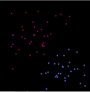
1. If the distribution of data looks like Fig. 1(a), it is very simple to separate it into two classes.
(All of the following graphs are all calculated by libsvm)

Fig. 1 (a)(b)

2. If the distribution of data looks like Fig. 2(a), it still makes sense.

Fig. 2 (a)(b)

For example, the horizontal axis represents the BMI of students, and the vertical axis is their sports performance.  This distribution can also be perfectly separated by SVM if a certain transformation is performed on the two axes.  For example, if you transform the BMI ratio to some score that represents the health of human body, the graph will look like Fig. 1 (which means "health score" is more suitable to describe such system).

3. If the distribution of data looks like Fig. 3(a), some red dots that surround by blue dots may be noises (i.e. data that is mistakenly labeled).  You know you want your algorithm to separate your data and gives the result like Fig. 3(b).  However, if your algorithm makes a fuss about such noises it would look like Fig. 3(c).  If this is the case, it will drag down the performance.

Fig. 3 (a) (b)

(c)

4. If the distribution of data looks like Fig. 4(a), this feature space may make no sense in my opinion.  This probably means this feature space is not adequate to describe such system.  If your algorithm tries hard and tends to separate these data into many small groups, it probably does it wrong.

Fig. 4 (a) (b)

In this case, you should probably abandon one of the features (or even both of them).  Or, find new features that describe the system well by setting some restrictions of your model (such as Regularization).  This may also be able to explain why Clustering can't give a better result than SVM:  Although the parameters of Clustering is quite a few (compare to the input data), trying to separate every data well is meaningless.

    Now, let us back to the high dimension feature space.  If your algorithm has many parameters that can fit into many circumstances (such as the fully-connected neural network), no matter current data is a noise or some of the features are poor to describe the system, it may get into trouble.  Instead, if one algorithm that can ignore some noises and take less of those features which does not help to classify objects, it may give a better result.

Multi-tasks in Convolution Neural Network (CNN) - the reuse of the extracted features

Overview

     This article will discuss one of the approaches to perform multi-tasks in computer vision: By extracting the features from a CNN and send those features to the traditional classification methods (such as SVM, Joint Bayesian... etc).  This article also shows the range of accuracy, so that one can judge if this approach satisfies his own purposes.

Motivation

     In some circumstances, we want more than one task is executed.  For example, supposed that we want to develop an APP that can recommend different products to different consumer groups by examining the age, gender, wear glasses... etc.  And judge their response to such advertisement by examining their facial expressions.  It seems that multiple CNN should be executed at a time.
     However, passing an image through one CNN is time-consuming.  Not to mention that there're so many tasks to be performed.  There should be other alternatives.

Introduction

     As shown below, the Convolution Neural Network (CNN) is usually composed of several Convolution Layer at the front of the network, as well as the Fully-Connected Layer at its end.

The former of the network are believed to perform the feature extraction (i.e. to extract the characteristic of such image). While the later layer, especially the Fully-Connected Layer, is believed to perform the classification of such image by using the previously derived features.
     Due to such characteristics of CNN, it is straightforward to replace the classification part (i.e. the Fully-Connected Layer) by the traditional classifiers (such as SVM).  For its efficiency and even its accuracy (see this article).
     In this article, we approach the multi-tasks by training a CNN for one task.  And perform other tasks by extracting features from that CNN and input those features to the traditional classifier to perform other tasks.  We believe that the features that used by one task may be close to the feature of the other task, if both of the tasks are similar to each other.

CNN + traditional classifiers

     In our case, we have at least three tasks to perform: to infer whether the user is smiling, wearing glasses, and the user's age.  We start from the DEX model (which is designed for age deduction), take features from the first the Fully-Connected Layer (so that the size of the features is large enough to do further processing) and finally, input those features to the traditional classifier (SVM in our cases).

Result

Age

      Since we do not re-train the CNN, the error of Age should remain the same (i.e. from its paper: MAE = 3.221).
-------------------------------------------------------------------------------------------------------------------------------------------------------------

      On the beginning of this project, our team has a heated discussion about whether the result of Smile-Task is more accurate than the Glasses-Task.  One might say that: since the glasses is more apparent than any other textures  of the human faces, the Glasses-Task should get the better result.  On the other hand, the other may say: since the DEX model is trained for detecting the human age, it might tend to only extract the features that relate to it (e.g. the wrinkle) and these features are more suitable for judging smiling.

Smile

      In this task, we only output two results: Smile or Not-Smile.  We collect about 3000 training data for each class to train SVM.
     The accuracy is around 88% which can be better if we train a model especially for detecting Smile.  However, this accuracy is suitable for our purpose.  Instead of letting users wait, some mistakes are tolerable.

Glasses

      In this task, we output three results: No Glasses, Glasses, and Sun Glasses.  We also collect around 3000 training data for each class.
      The accuracy is only around 84%.  Looks like the Smile-Task win!  To give a brief interpretation after the result, this might due to the DEX model is trained for predicting age.  Therefore, the later parts of the network might tend to ignore some features that belong to the glasses, since wearing a glasses does not change the age of a human.
      Furthermore, the result of glasses may get better if we extract features from the former layers.  However, since the features of the former layer is quite large (10 times as many features than we have used) and will drag down the efficiency.

Conclusions

    It's possible to use features that extracted by CNN that is trained for another purpose.  And the performance is around 80%~90% depend on whether current task is close to the original task (for which the CNN is designed).

Taiwan ancient buildings recognition by Convolution Neural Network

Overview

       The Alex net is applied to recognize 4 different types of Taiwan ancient buildings in this article.

Motivation

      I'm new to Deep Learning, so I want to do some exercise to warm up.  And since it would be interesting and meaningful to combine the technology together with the culture, I apply the Alex net to recognize 4 different types of Taiwan ancient buildings.

Introduction

     The ancient buildings in Taiwan can be categorized into 4 types:

1. The traditional Chinese buildings:  Many of Taiwanese are successors of the immigration who emigrated from China about hundred years ago.  Therefore, many old buildings are ancient Chinese buildings.  The following figure shows the traditional residence.

2. The traditional Japanese buildings:  Taiwan has been colonial ruled by Japan for about half of the century. Therefore, there're many traditional Japanese buildings left.  The following figure shows the Japanese temple located in Taoyuan.

3. The baroque style buildings:  During the Japanese colonial period, several government buildings are designed as the Japanese Baroque style.  These buildings are popular in Japan during the Meiji period. Thus, this category is labeled as Japanese modern in the present work.  The most famous building of this style might be the Presidential Palace of Taiwan, as shown follows.

4. The modern Taiwan buildings:  The word "modern" here refers to those buildings that constructed during the Early Revival Period.  I'm not quite a fan of these kinds of buildings.  However, these buildings still in everyone's childhood memory.  Thus, these buildings are also recognized by the network.

Data Sets

       The collection of data is very time-consuming. And since there are only countable historic buildings in Taiwan as well as not every building in these kinds are posted to the internet, I suddenly ran out of data to train the net.  Therefore, some of the buildings in Chinese and Japanese are also collected.
       After all, I spend a whole data to collect all of the following data!  However, the training set seems too few to train an Alex net, though...
      The collected data are listed below (25% of these data are used to calculate the validation):
Traditional Chinese Buildings: 159
Traditional Japanese Buildings: 152
Modern Japanese Buildings: 169
Modern Taiwan Buildings: 119

Result

       The training result is shown as follows.  After 30 epoch, the final accuracy (validation set) is 66%.

Several results in the test set are shown below:

       Although the training data are quite insufficient, the result seems acceptable: up to 2/3 buildings are classified correctly.  And it might get better performance if more and more data are included.  Also, the Alex net seems to be capable of solving problems like this.  Therefore, it's more reasonable to collect more data than design more complex neural network if one want to improve the predictions.